Introduction
FALCON is a FEM code written in Fortran90 used to study large-scale geodynamics system, such as continental rifting and subductions. Here you can download the .pdf file with the complete description of all the fetures implemented in the code and all the benchmarks performed. The Gihub repository of this project can be found here and you can download the .zip file containing all of the files at this link.
Table - List of the features implemented in FALCON and of the benchmarks performed.
Features implemented
Governing equations
The code is written in Fortran90 and uses the finite element method (FEM) with quadrilateral $Q_1\times P_0$ elements (continuous bilinear velocity and discontinuous constant pressure), associated with MUMPS (Amestoy et al., 2001, 2019) that is a software package for solving systems of linear equations by means of a direct method. Since $Q_1\times P_0$ elements do not satisfy Ladyzhenskaya, Babuska and Brezzi (LBB) stability condition (Donea and Huerta, 2003), elemental pressure is elaborated in post-processing to avoid spurious pressures by means of a double interpolation to smooth the pressure. The thermo-mechanics of crust-mantle systems is described by means of the conservation of mass, momentum and energy equations. The time step dt is chosen in according to Courant-Friedrichs-Lewy (CFL) condition (Anderson, 1995).
Lagrangian markers
Elemental properties (density, viscosity, thermal conductivity, specific heat and thermal expansion) are related to the composition of each element, determined by means of Lagrangian markers that are characteristic of different materials in the domain. The advection of the markers is performed by either a $2$nd-order or a $4$th-order Runge-Kutta in space, interpolating the velocity field on each marker by means of the shape functions. The interpolated velocity is then corrected by means of the Conservative Velocity Interpolation (CVI; Wang et al., 2015). The initial distribution of the markers is created using the open-source code library Geodynamic World Builder (Fraters et al., 2019). During the simulation, each marker carries memory of temperature, pressure and accumulated strain and the number of markers contained in each element is maintained between a minimum and a maximum by adding or deleting random markers inside the elements. In this way elements are never empty and maintain a number of markers inside a prefixed range.
Momentum and energy equations
The code implements a so-called penalty formulation for which the flow is not truly incompressible but very weakly compressible. This allows to eliminate the pressure from the momentum equation that is then solved for the velocity field, while the pressure can be recovered as a post-processing step. One strong requirement is that the penalty coefficient $\lambda$ must be many orders of magnitude larger than the dynamic viscosity $\eta$ (typically between $5$ and $8$ orders of magnitude).
The stabilisation of the advection term of the energy equation, needed to avoid possible oscillations in the thermal solution in the case when advection dominates over diffusion, is implemented by means of a streamline-upwind Petrov–Galerkin (SUPG) method, for which the advection term is modified follows the discussion in Thieulot (2011) and Thieulot (2014).
Non-linear rheologies
Non-linear rheologies are implemented combining viscous creep (dislocation and diffusion) and plastic yielding. The viscous creep $\eta_{\rm cp}$ is calculated as the harmonic average between $\eta_{\rm df}$ and $\eta_{\rm ds}$, while the plastic yielding is implemented rescaling $\eta_{\rm cp}$ in order to limit the stress below the yield stress $\sigma_{\rm y}$ determined following the Drucker-Prager criterion. Plastic yielding and viscous creep are then combined to obtain a viscoplastic viscosity $\eta_{\rm vp}$ assuming that they are independent processes and the effective viscosity $\eta_{\rm eff}$ is capped by the minimum and the maximum viscosity to avoid extremely low or high viscosities. Viscous creep and plastic yielding are non-linear rheologies because of their dependence on the velocity field through pressure and strain rates. Therefore, the solution is determined by means of Picard-type iterations, until convergence of the velocity field. The temporal evolution of the accumulated strain $\epsilon$ has been implemented as in Fuchs and Becker (2019, 2021).
Strain softening
Strain softening is taken into account for both viscous creep and plastic viscosity by means of the accumulated strain ϵ memorised by each marker. Softening in the viscous creep determines a linear decrease of ηvc by means of a viscous strain softening factor WS, while plastic softening is simulated with a linear decrease of internal friction angle $\phi$($\epsilon$) and cohesion C($\epsilon$). The marker strain is computed by means of the deformation tensor. For each marker, the displacement gradient tensor $F$ is computed, then polar decomposition is carried on to write $F$ as product of stretch and rotation ($F=V \cdot R$). The principal stretches $\lambda_{1,2}$ are then computed as the eigenvalues of $V$, and the eigenvectors represent the directions of maximum stretch. The angle of rigid rotation is then calculated from $R$.
Sticky air and free surface
The Earth’s surface can be treated by means of either the so-called sticky-air or a true free surface method, both of them implemented in the code. In the sticky-air method the surface is approximated with the introduction of a buoyant layer with a viscosity at least four orders of magnitude lower than the crust (Schmeling et al., 2008; Crameri et al., 2012) and the interface between lithosphere and air is defined using a chain of passive markers that are advected as the Lagrangian markers. In the true free surface case the top boundary is assumed stress-free and velocities are not fixed. In this case topography variations are described by vertical deformations of the mesh that depend on the velocity field of the nodes that identify the free surface, while horizontal deformations are not taken into account. This procedure is known as the Arbitrary Lagrangian-Eulerian (ALE) method and its implementation follows the technique described in Thieulot (2011) . The stability algorithm proposed by Kaus et al. (2010) is implemented to avoid instabilities due to high density differences at the free surface when using too large time steps.
Phase changes and hydration
Variations of effective density, specific heat and coefficient of thermal expansion during the evolution of crustal and mantle materials at different pressure-temperature ($P$-$T$) conditions are computed by means of MAGEMin (e.g., Riel et al., 2022). In the case that hydration is switched on, the amount of bound and free water is memorised by each marker, following the implementation of Quinquis and Buiter (2014); hydration and dehydration processes are related to the amount of bound water of each marker and to the maximum amount of water it can transport, i.e. if the amount of bound water exceeds the maximum amount of water, the marker dehydrates and releases free water that can hydrates under-saturated markers. Bound water is advected together with the markers, neglecting the effect of bound water diffusion, while free water simply migrates vertically and is not coupled to the solid-phase flow of the mantle wedge.
Mantle melting
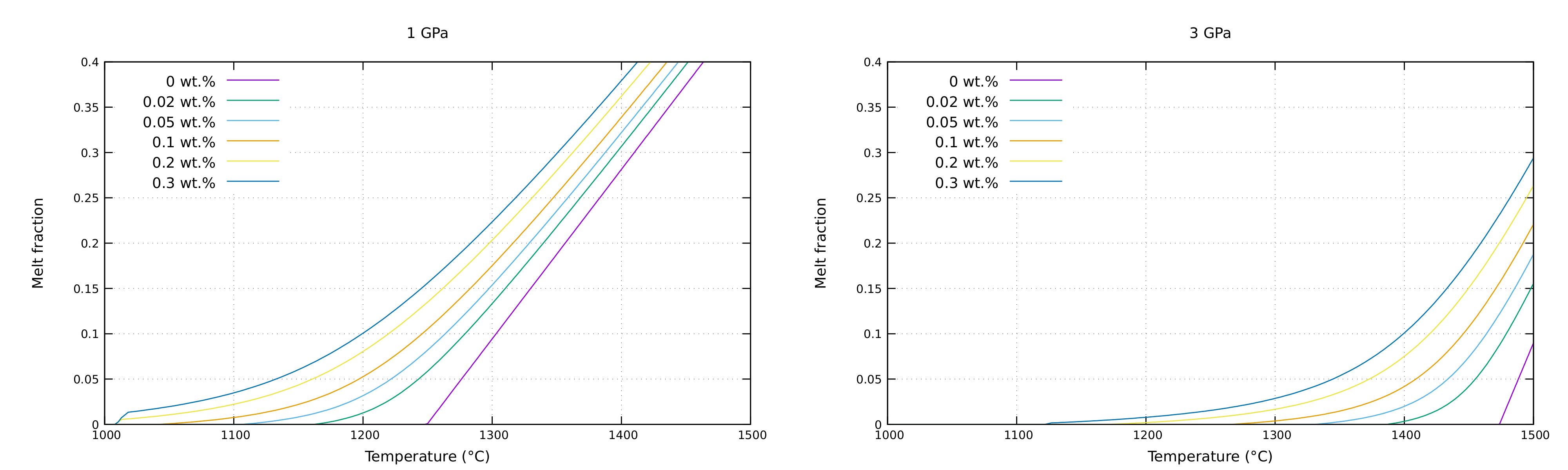
Melt fraction in the mantle depends on temperature ($T$), pressure ($P$) and the water content in the melt (in $wt$.%). The determination of the melt fraction is implemented as explained by Katz et al. (2003). In case of melting, viscous creep viscosity and effective density are modified according to Wang et al. (2016).
Benchmarks
This is a brief description of the benchmarks performed to verify that FALCON correctly solves a wide range of problems, as in the Table below. The Gihub repository with the results of all the benchmarks can be found here, and you can download the .zip file containing all of the files at this link.
Stokes flow
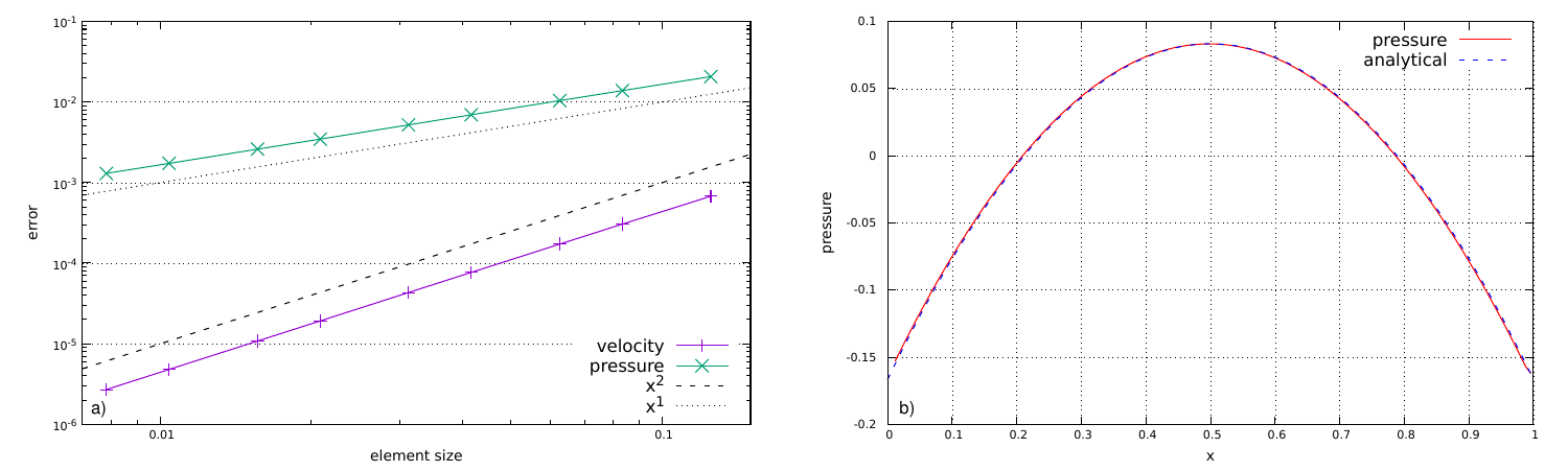
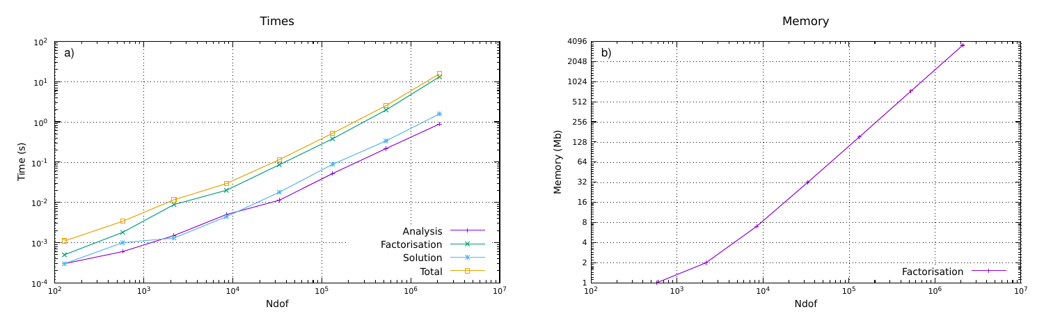
This experiment is performed as explained by Donea and Huerta (2003). The problem consists of determining velocity field $(u,v)$ and pressure $P$ in case of a manufactured solution with prescribed body forces. The domain is a unit square a constant viscosity and the penalty parameter is set to $10^7$. Velocity boundary conditions are set to no slip on all boundaries. The problem is performed for different grid resolution between $8\times 8$ and $1024\times 1024$ elements.
Zalesak disk
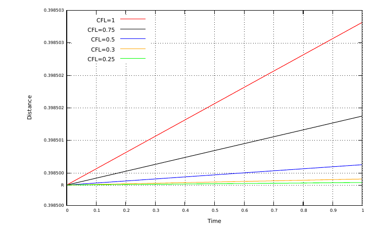
This experiment is performed as explained by Zalesak (1979). The benchmark is performed in a unit square domain with a grid resolution of $32\times 32$ elements and values of Courant number (CFL) between $0.25$ and $1$. The velocity field is prescribed in the entire domain. At $t=0$, the disk is centred at position $(0.5; 0.75)$ with a radius $R=0.15$ and has a vertical fissure $0.05$ wide and $0.2$ high.
Conservative Velocity Interpolation
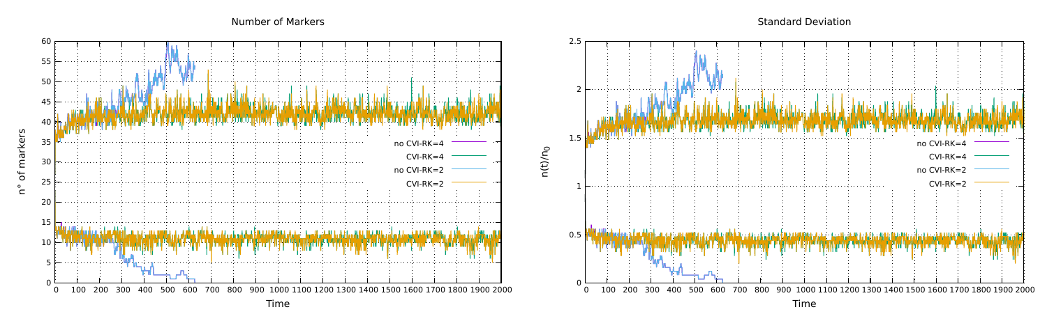
The Conservative Velocity Interpolation (CVI) correction is checked by means of the Stokes flow experiment, as explained in FIELDSTONE (Stone 30). The advection of Lagrangian markers is performed using either a $2$nd-order or a $4$th-order Runge-Kutta scheme with CFL=$0.5$ and an initial random distribution of $25$ markers per element.
Poiseuille flow
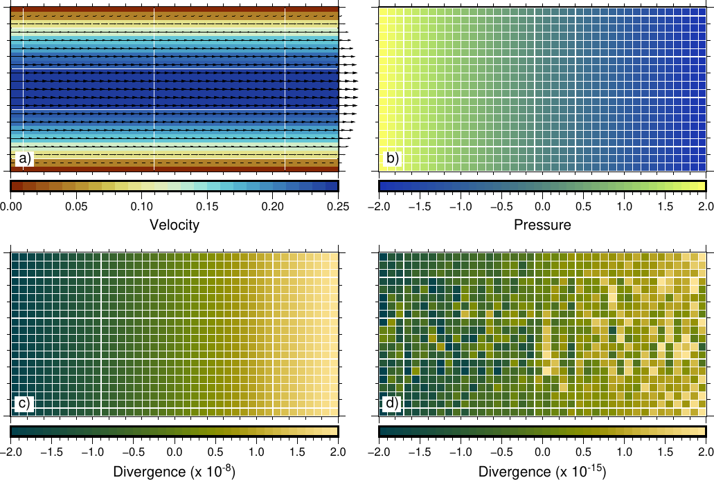
This experiment is performed as explained by Thieulot (2014). The domain is a rectangle with $L_x=2$ and $L_y=1$, constant density and viscosity, gravity acceleration equal to $0$ and the penalty parameter is $10^8$. The grid is composed by $40\times 20$ elements. Velocity boundary conditions are set to no slip at the top and the bottom, and a parabolic profile is imposed on the sides, with $u=y(1−y)$ and $v=0$.
Instantaneous 2D sphere
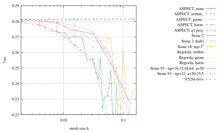
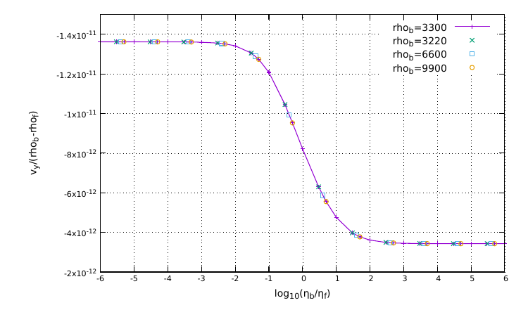
The experiment is performed as explained in FIELDSTONE (20.24). The domain is a unit square with $g_y=-1$. The fluid has constant density and viscosity. The sphere is in the middle of the domain with a radius $R=0.123456798$ with constant density and viscosity higher than the fluid. Different types of velocity boundary conditions have been tested with grid resolutions between $16\times 16$ and $512\times 512$ elements and different average schemes for the viscosity (harmonic, geometric and arithmetic).
Rayleigh-Taylor experiment
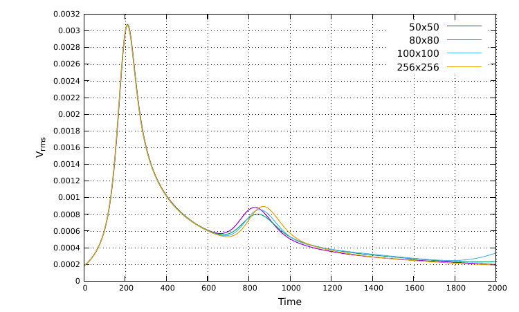
This experiment is performed as explained by Van Keken et al. (1997). The domain has $L_x=0.9142$ and $L_y=1$, and $g_y=-1$. Two fluids with same constant viscosities and different densities are distributed in the domain, with the lighter fluid at the bottom. The initial interface between the fluids is given by $y(x)=0.2+0.02$ cos(πx $L_x$). The experiment is performed with grid sizes between $50\times 50$ and $256\times 256$ elements. Velocity boundary conditions are set to no slip at the top and the bottom, and to free slip at the sides of the domain.
Falling block
This experiment is performed as explained by Gerya and Yuen (2003) and Thieulot (2011). The domain is square with $L_x=L_y= 500~ km$ and the grid is composed by $50\times 50$ elements with $25$ markers in each element. The block is initially centred at $x=250~ km$; $y=400~ km$ and has a size of $100\times 100~ km$. The fluid surrounding the block has constant viscosities and densities. The benchmark tests with different viscosities and densities of the block, with higher density than the surrounding fluid. Velocity boundary conditions are set to free slip conditions on all sides of the domain.
2D Stokes sphere
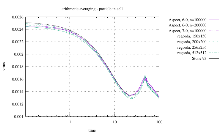
This experiment is performed as explained in FIELDSTONE (20.25), in a unit square domain with $g_y=−1$. The sphere has constant densities and viscosities hogher than the surrounding fluid and it is initially centred at $(0.5; 0.6)$ with radius $R = 0.123456789$. The fluid surrounding the sphere occupies the domain for $y\le 0.75$, while for $y>0.75$ there is air. Velocity boundary conditions are set to free slip on all sides. The Courant number is set to $0.25$. The experiments run for $200~ s$ using grid resolutions from $150\times 150$ to $512\times 512$ elements, with $25$ randomly distributed markers per element, and for different average schemes for the viscosity. The interface between the fluid and the air is tracked by means of the markers chain.
Stabilisation algorithm
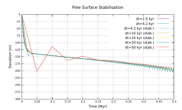
This experiment is performed as explained by Kaus et al. (2010). The domain is square with $L_x=L_y=500~ km$ and a grid resolution of $200\times 200$ elements, each of them containing $16$ markers. A buoyant fluid is overlain by a denser fluid. The initial interface between the fluids has an initial sinusoidal shape of $5 ~km$ amplitude. Velocity boundary conditions are set to free slip conditions at the sides and no slip at the bottom, while the top is free surface. The experiment is performed with various fixed time steps.
Topography relaxation
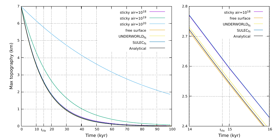
This experiment is performed as explained by Crameri et al. (2012). The domain is rectangular with $L_x=2800~ km$ and $L_y=700~ km$ in case of free surface and $L_y=800~ km$ in case of sticky air. The grid is composed by $256\times 64$ elements for the free surface $560\times 320$ elements for the sticky air. For both cases, there is a mantle of $600~ km$ thickness overlain by a highly viscous cosine-shaped lithosphere with thickness between $93$ and $107~ km$. Velocity boundary conditions are set to no slip at the bottom and free slip at the sides of the domain. In case of sticky air, velocities on top are set to free slip conditions.
Spontaneous subduction
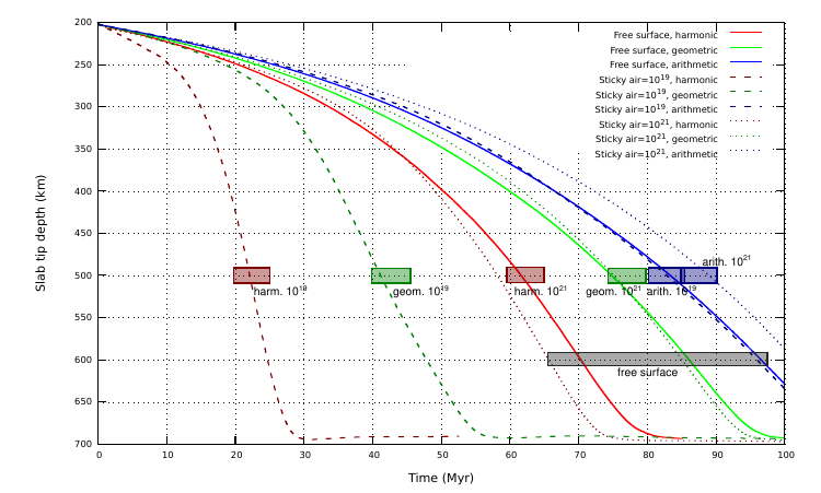
This experiment is performed as explained by Schmeling et al. (2008), with both a sticky air and a true free surface and using different average schemes for the viscosities. The domain is rectangular with $L_x=3000~ km$ and $L_y=700~ km$, a grid resolution of $256\times 64$ elements with $50$ markers per element and Courant number of $0.01$. At the beginning of the simulation, a denser $100 ~km$-thick lithospheric layer is located at the top of the domain for $x$ between $1000$ and $3000~ km$. In addition, a $200~ km$-depth lithospheric slab is already subducted in the mantle in order to have a spontaneous subduction. In case of sticky air, a $50~ km$-thick air layer overlie the mantle. Velocity boundary conditions are set to free slip on the sides and on the bottom of the domain. In case of sticky air, velocities on the top boundary are set to free slip conditions as well.
Slab detachment
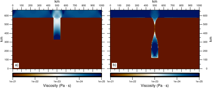
The slab detachment benchmark is performed as explained by Schmalholz (2011) and Glerum et al. (2018). The domain is rectangular with $L_x=1000~ km$ and $L_y=660~ km$ and a grid resolution of $256\times 256$ elements. A denser non-linear viscous T-shaped layer is placed at the top of the domain and surrounded by a linear viscous fluid. The top layer is $80~ km$-thick and a $250~ km$-long and $80~ km$-wide slab is placed at $x=L_x/2$. Velocity boundary conditions are set to free slip at the top and the bottom, and to no slip at the sides of the domain.
Indenter
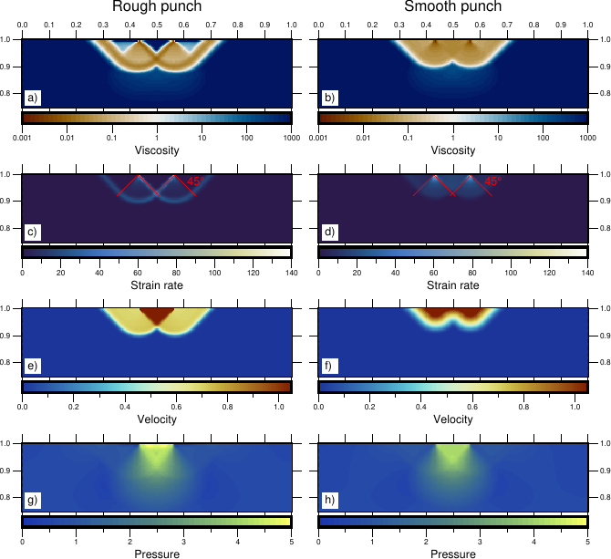
The indenter benchmark is performed as explained by Thieulot et al. (2008) and Glerum et al. (2018). The indenter benchmark simulate a rigid punch on a purely plastic von Mises material, for which exists an analytical solution. The domain is a unit square with a grid resolution of $256\times 256$ elements. The gravity acceleration is set to $0$. Velocity boundary conditions are set to no slip at the bottom and free slip at the sides of the domain. The top of the domain is open with the exception of the central portion (punch area) with width $wp=0.125$, where $v_y=−1.05$ and $v_x$ is fixed either to $0$ (rough punch experiment) or free (smooth punch experiment).
Brick
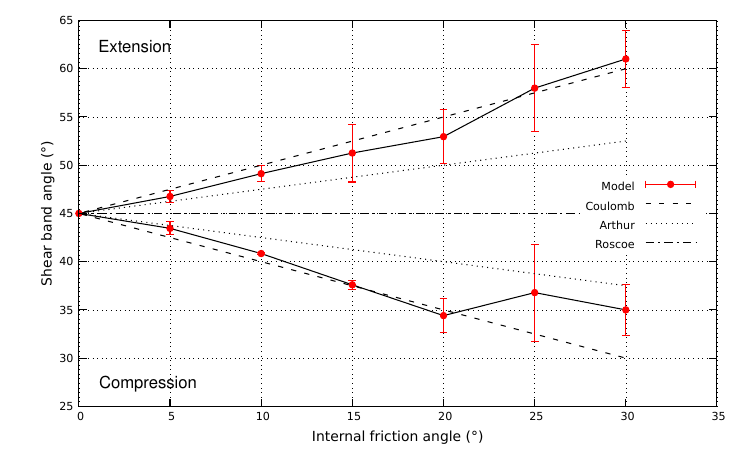
The experiment is perfomed as explained by Glerum et al. (2018) to verify the correctness of the pressure-dependent plasticity for different angle of internal friction. The domain is rectangular with $L_x=40~ km$ and $L_y=10~ km$ and a grid resolution of $512\times 128$ elements. The maximum number of non-linear iterations is set to $1000$. A $800~ m$-wide and $400~ m$-height inclusion is placed at the bottom of the domain at $x=L_x/2$. The inclusion is surrounded by a non-linear viscous medium. Velocities are set to free slip conditions at the bottom of the domain and the top is open. Velocities on sides of the domain are fixed to $v_x=\pm 2\times 10^{−11}~m~ s^{−1}$ and $v_y=0$. The experiment is performed in compressional and extensional contexts with an angle of internal friction of the non-linear medium variable between $0°$ and $30°$.
Integrated deformation
This benchmark is composed by $4$ experiments characterised by different velocities imposed. For all the experiment the domain is a square of size $L_x=L_y=1$, discretised by $40\times 40$ elements. The velocities for the $4$ experiments are imposed as follows:
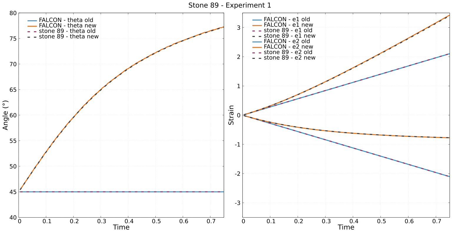
Experiment 1: $u(x,y)=0$; $v(x,y)={\rm erf}[A(x-L_x/2)]$
Experiment 2: $u(x,y)=0$; $v(x,y)=y$
Experiment 3: $u(x,y)=y$; $v(x,y)=x$
Experiment 4: $u(x,y)=2(-x+L_x/2)$; $v(x,y)=y-L_y/2$
The simulations are performed for $51$ timesteps, calculated by using CFL=$0.2$. The results for Experiment $1$ are shown comparing directions and values of the principal strains, calculated with the integrated deformation method (new) and the standard method of integrating the strain (old).
Advection stabilisation
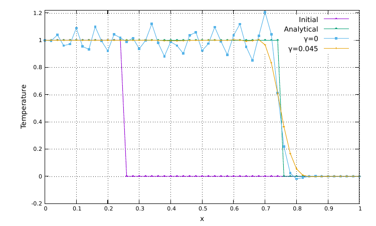
The 1D advection problem proposed by Donea and Huerta (2003) and Thieulot (2011) is performed to verify the effectiveness of the SUPG method to stabilise the advection term of the energy equation. The domain is a $1$D segment with $L_x=1$ composed by $50$ elements and a discontinuity in the thermal field placed at $x=0.25$. Temperature is set to $1$ for $x \le 0.25$ and to $0$ for $x > 0.25$. Velocity is set to $u_x=1$ in the entire domain. The simulation is performed for $250$ time steps, with $dt = 0.002$, so the thermal discontinuity should be at $x = 0.75$ at the end of the simulation. Temperature profiles at the end of the simulation are function of the dimensionless coefficient $\gamma = \tau u_x/h$.
Simple shear heating
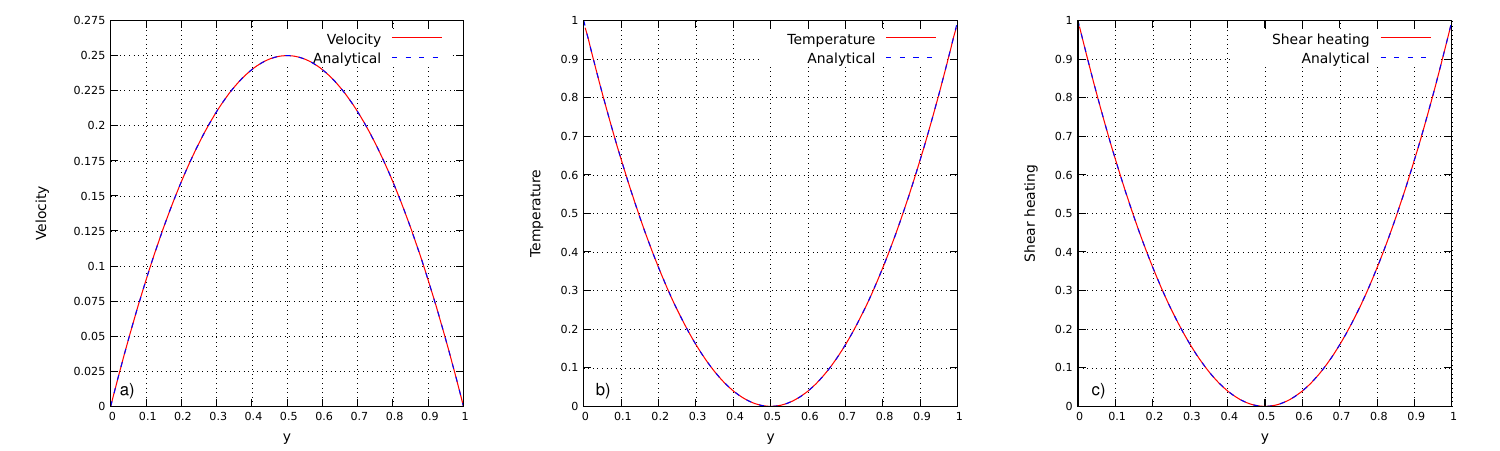
This exercise is performed in an unit square domain composed by $128\times 128$ elements. The velocity field is prescribed on the entire domain with $u_x=(L_y−y)y$; viscosity, density and specific heat are fixed to $1$, while thermal conductivity and radiogenic energy are fixed to $0$. Therefore, the energy equation can be simplified and fixing $T(t=0)=0$, the temperature can be find as $T(t)=H_s t$, where shear heating $H_s$ can be calculated as $H_s(x,y)=(1−2y)^2$.
Shear and adiabatic heating
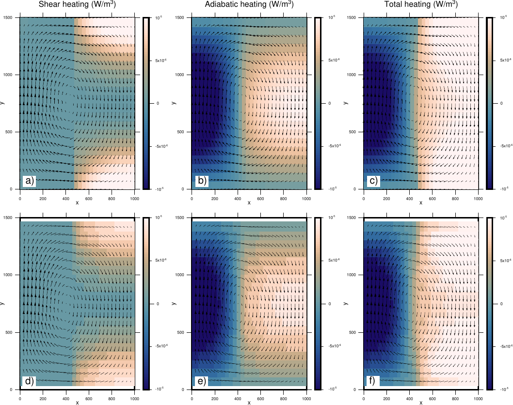
This problem is performed as presented in Exercise $9.4$ in Gerya (2010). Two materials are vertically separated in a rectangular domain with $L_x=1000 ~km$, $L_y=1500 ~km$ and a grid resolution of $30\times 20$ elements. Constant thermal coefficient expansion $(\alpha=3\times 10^{−5}~ K^{−1})$, temperature $(T=1300~ K)$ and gravity acceleration $(g_y=−10~ m~s^2)$ are assumed in the whole domain. Fluid $1$ on the left side of the domain has lower densities and viscosities with respect to fluid $2$ on the right side of the domain. Velocity boundary conditions are set to free slip on all sides of the domain.
Mantle convection
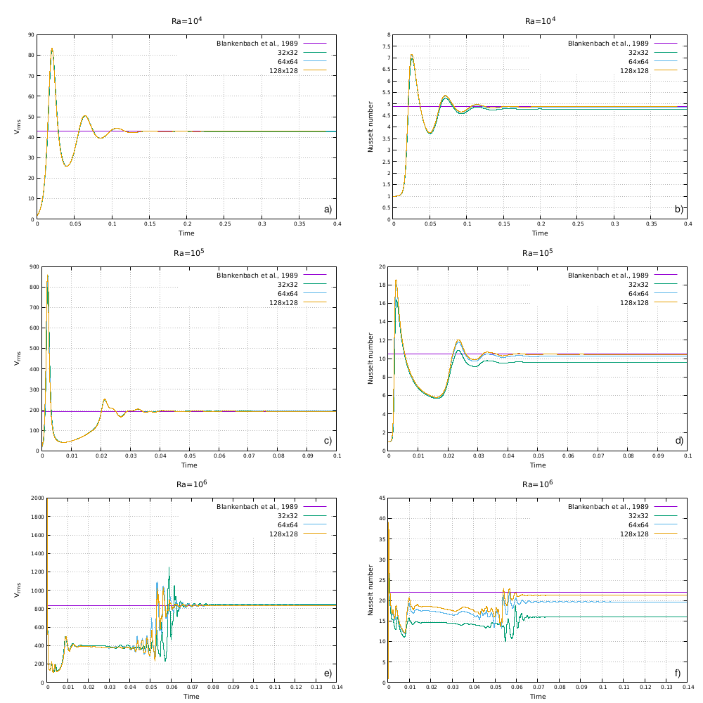
This problem is performed as presented by Blankenbach et al. (1989)(constant viscosity cases), in a $2$D unit square domain with gravity acceleration $g_y=10^{10}~Ra$. The experiment is performed with three different Rayleigh numbers $(Ra=10^4$, $10^5$ and $10^6)$ and with different grid resolution (between $32\times 32$ and $128\times 128$ elements). The fluid has constant viscosity, initial density, heat capacity, thermal conductivity $(\eta =\rho_0=C_p=k=1)$, reference temperature $(T_0=0)$ and thermal expansion coefficient $(\alpha=10^{−10})$. Temperatures are set to $0$ on top and $1$ on bottom of the domain. Velocity boundary conditions are set to free slip on all sides. The initial temperature field is given by $T(x,y)=(1−y)+0.01 {\rm cos}(\pi x) {\rm sin}(\pi y)$.
Visco-plastic mantle convection
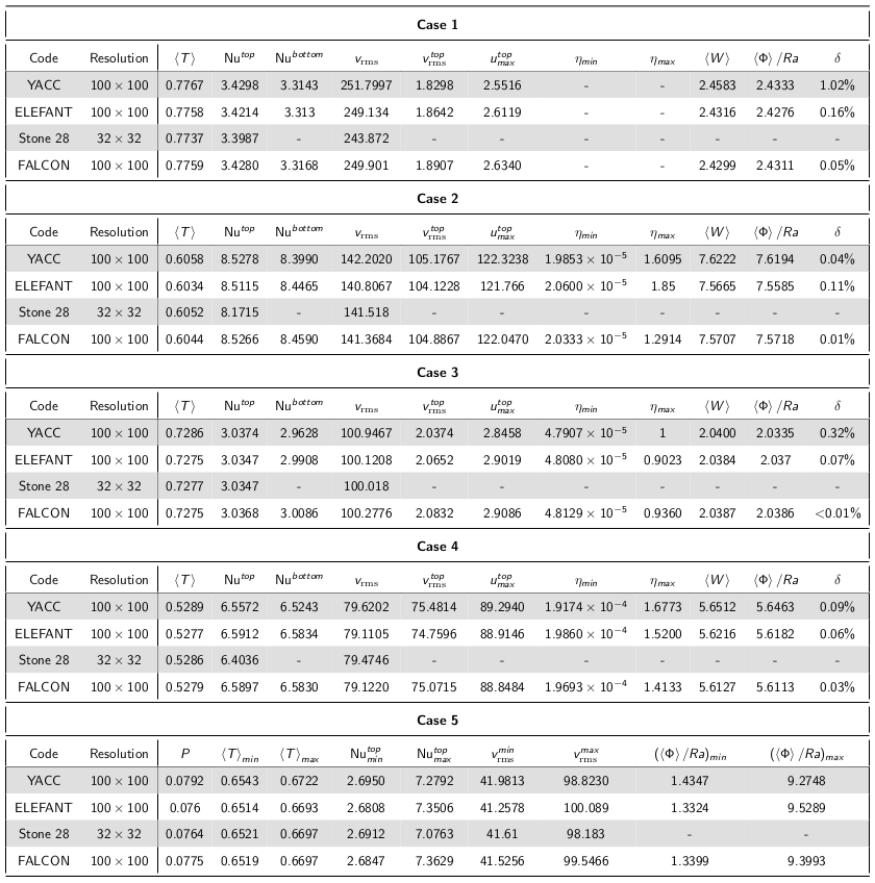
This benchmark is performed as Cases $1$-$5$a described in Tosi et al. (2015) in a $2$D unit square domain with two different grid resolutions of $32\times 32$ and $100\times 100$ elements. Reference viscosity, reference density, heat capacity, thermal conductivity and thermal expansion coefficient are fixed to a constant value of $1$ $(\eta_0=\rho_0=C_p=k=\alpha=1)$, while the gravity has been chosen as $g_y=10^2$, in order to obtain a Rayleigh number $Ra=10^2$. Temperatures are set to $0$ on top and $1$ on bottom of the domain. Velocity boundary conditions are set to free slip on all sides. The initial temperature field is given by $T(x,y)=(1−y)+0.01 {\rm cos}(\pi x) {\rm sin}(\pi y)$. The viscosity field $\eta$ is calculated as the harmonic average between a linear part $\eta_{\rm lin}$ that depends on temperature only or on temperature and depth $y$ and a nonlinear-plastic part $\eta_{\rm pl}$ that depends on the strain rate $\epsilon$. See Tosi et al. (2015) for more details.
Thin layer entrainment
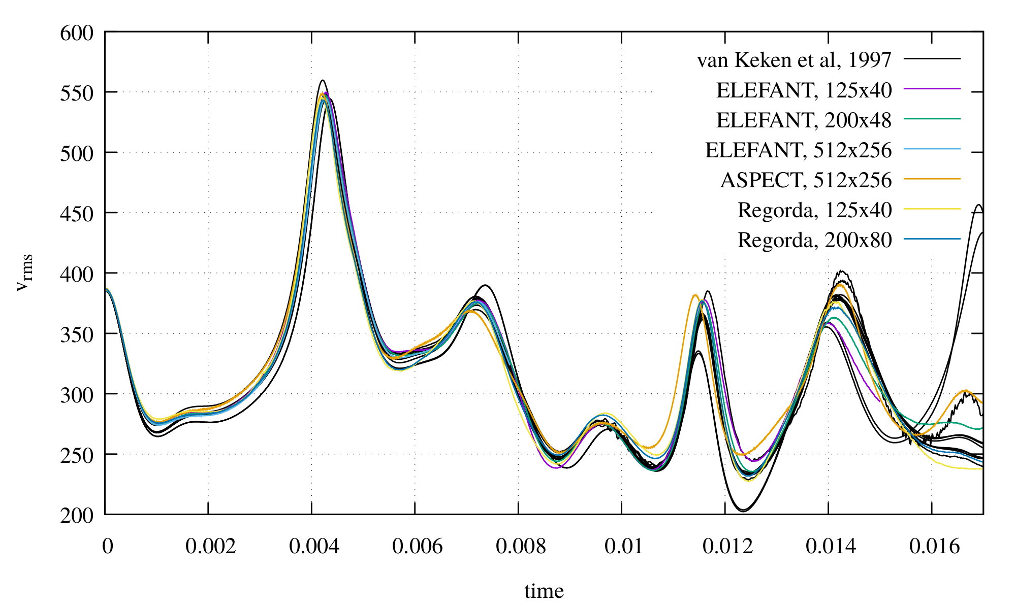
This experiment is performed as originally proposed by Van Keken et al. (1997) with two incompressible fluids in a rectangular domain with $L_x=2$ and $L_y=1$ and gravity acceleration $g_y=10^{10}~ Ra$. The Rayleigh number and the compositional Rayleigh number are fixed to $Ra=300000$ and $Rc=450000$, respectively. Both fluids have constant viscosity, thermal conductivity, specific heat $(\eta=\rho=C_p=1)$ and thermal expansion coefficient $(\alpha=10^{−10})$. Fluid $1$ has a density $\rho_1=1$, while fluid $2$ is denser $(\rho_2=\rho_1+1.5\cdot 10^{−10})$ and is placed at the bottom of the domain, for $y\le 0.025$. Temperature are set to $0$ on top and $1$ on bottom of the domain. Velocity boundary conditions are set to free slip on all sides of the domain. See Van Keken et al. (1997) for details about the initial temperature field. The experiment is performed with two grid resolution ($125\times 40$ and $200\times 80$ elements), with $100$ markers per element and Courant number of $0.25$.
Hydrated sinking cylinder
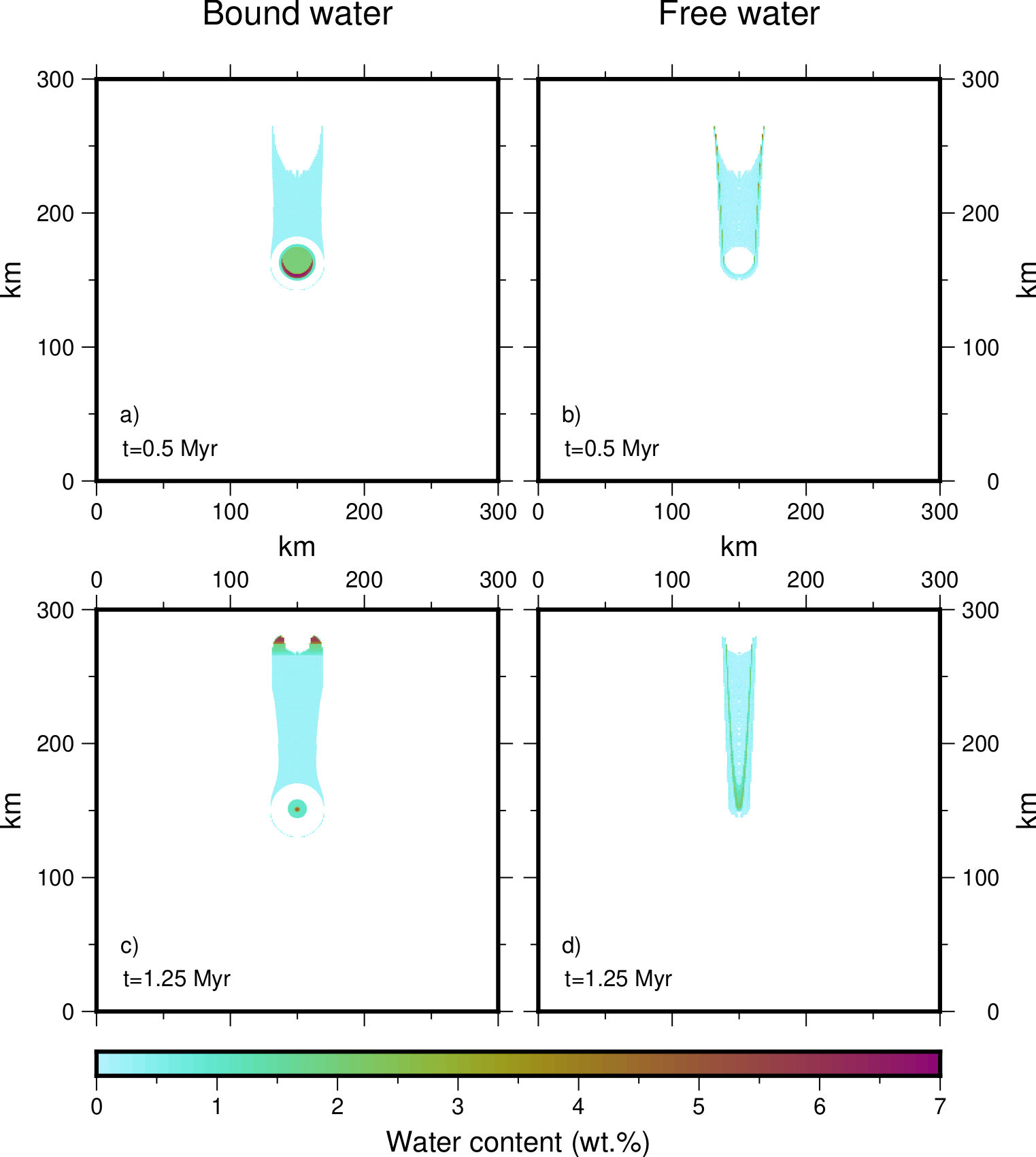
This experiment is performed as explained in Quinquis and Buiter (2014) and simulates the sinking of a cold, hydrated cylinder into a warm, dry mantle. The domain is square with $L_x=L_y=300 ~km$, a grid resolution of $300\times 300$ elements and $25$ markers per element. The sinking cylinder is located at $x=150 ~km$ and $y=170 ~km$ with a radius of $20~ km$ and has $\rho_c=3250~ kg~ m^{−3}$, $\eta_c=1\times 10^{23}~ Pa ~s$, a thermal conductivity $k_c=4.5~ W ~m^{−1}~ K^{−1}$, a specific heat $C_{pc}=1250~ J~ kg^{−1}~ K^{−1}$; the surrounding mantle has $\rho_m=3200 ~kg~ m^{−3}$, $\eta_m=1\times 10^{20}~ Pa~ s$, a thermal conductivity $k_m=105~ W~ m^{−1}~ K^{−1}$ and specific heat $C_{pm}=1250~ J~ kg^{−1}~ K^{−1}$; a $58 ~km$-thick lithosphere overlies the mantle and has $\rho_l=3200~ kg~ m^{−3}$, $\eta_l=1\times10^{23}~ Pa~ s$, a thermal conductivity $k_l=4.5~ W~ m^{−1}~ K^{−1}$, $C_{pl}=750~ J~ kg^{−1}~ K^{−1}$ and a thermal diffusivity of $1\times 10^{−6}~ m^2~ s^{−1}$. Velocity boundary conditions are set to free slip on all sides of the domain. Temperature increase linearly in the lithosphere, from $0°$ to $1300°C$, and in the mantle, from $1300°$ to $1360.5°C$. The initial temperature of the cylinder is fixed to $400°C$. Throughout the evolution, temperature is fixed to $0°$ and $1360.5°C$ at the top and bottom of the domain, respectively. The initial bound water content is imposed at $2$ $wt$.% in the cylinder and at $0$ $wt$.% in both the mantle and the lithosphere. The maximum amount of water in the mantle is fixed to $0.2$ $wt$.%, while maximum water content in the cylinder and in the lithosphere is function of pressure and temperature and is calculated using a serpentinized harzburgite with Perple_X, as in Quinquis and Buiter (2014).
Experimental melting curves
This instantaneous experiment is performed in order to recreate isobaric melting curves, as function of temperature, bulk water and content of water in the melt, to compare with melting curves obtained by Katz et al. (2003). The domain is square with $L_x=L_y=100 ~km$, a grid resolution of $100\times 100$ elements and $25$ markers per element. Density is set in the entire domain to $3300 ~kg ~m^{−3}$ and temperature increases from the sides to the centre from $1000°$ to $1500°C$. The experiment is performed for bulk water contents from $0$ to $0.3$ $wt$.%.